Cluster Tool Simulation Group

Results

In order to demonstrate the benefits of using our tool, we performed a sample scheduling analysis, which acts as a proof-of-concept (POC) for the use of the simulation tool.

In this analysis we created multiple lot sequences with a random generator and used three simple scheduling algorithms (Shortest Job Greedy, Longest Job Greedy, and Permutation Algorithm) to generate recipe sequences to input into our simulation tool. Since the three algorithms provide recipe sequences with different processing times, the goal was to compare the effects of the different sequences on the life of the ion source.

It must be noted that the deterioration effect of each recipe is user defined; users can obtain these effects from historical data. For this sample study, we assumed that the deterioration due to recipes was random, with a normal distribution. Therefore, in this study, the sequences were run multiple times to sample the life of the ion source, which is affected by random deterioration.

Data for the total processing time and the remaining ion source life was recorded at the end of the simulation runs. Then, the averages of the total processing time and the remaining source life were calculated for each recipe sequence generated by the three scheduling algorithms. Table 9.2.6 shows these results for 30 sequences.

Table 9.2.6

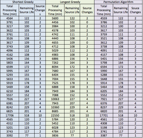
Figure 9.2.1, presented below, shows the average total process time versus the remaining source life for each recipe sequence, for the three scheduling algorithms. In this figure, each data point is represented by a diamonds, squares or triangles, which correspond to the shortest greedy algorithm, longest greedy algorithm, and the permutation algorithm, respectively. More specifically, each data point represents a sequence that was run by following one of the three scheduling algorithms. Furthermore, each data point shows how fast a given sequence was completed and the remaining source life after the processing was completed.

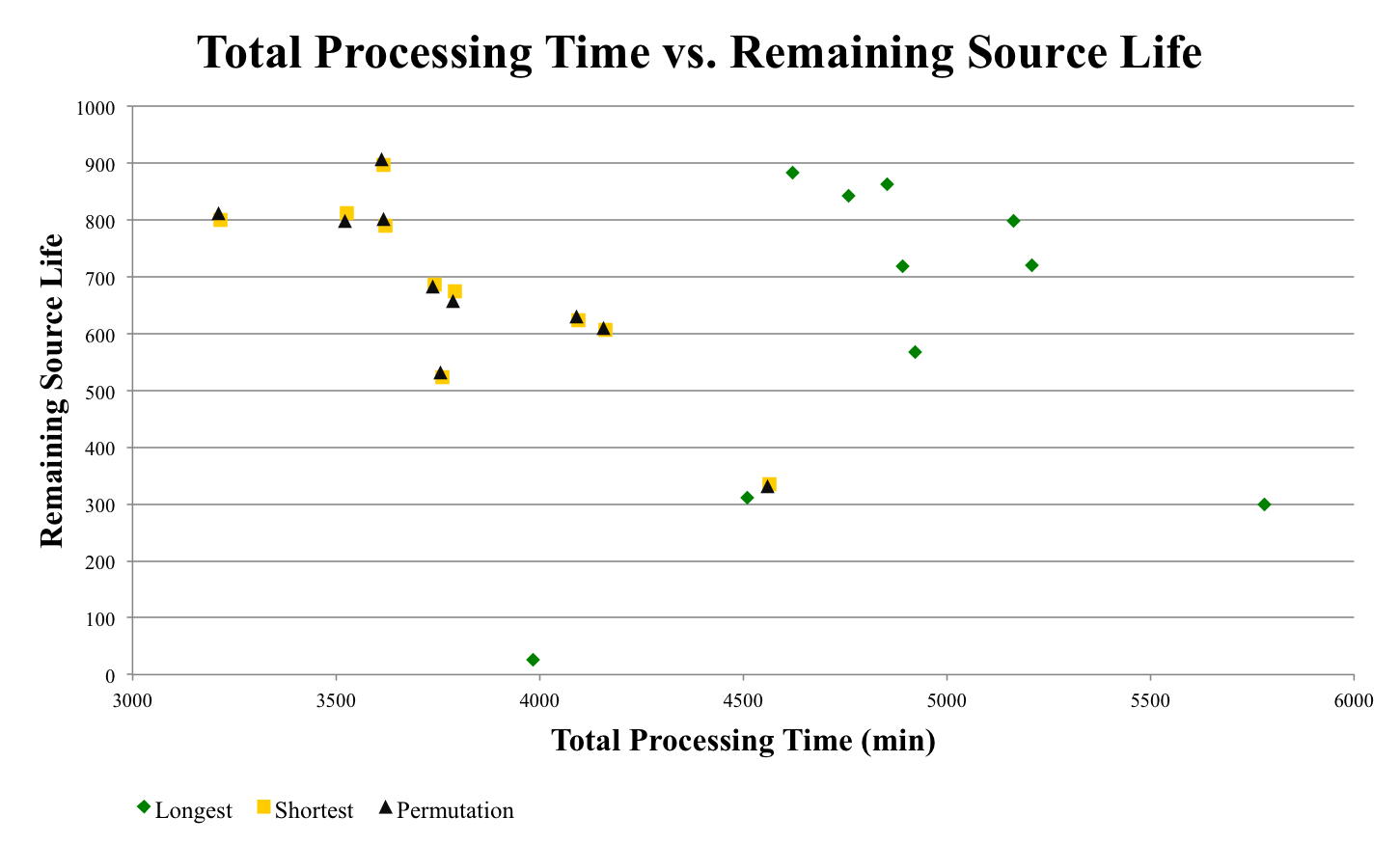
Figure 9.2.1: Processing Time vs. Remaining Source Life

In order to take a closer look at the data, we have presented the results for the total processing time and the remaining life of the ion source in separate plots. Figure 9.2.2 shows the average total processing time for ten of the sequences we ran. Here, it is evident that the longest greedy algorithm has the slowest processing times. Additionally, we can see that the shortest greedy and the permutation algorithms are very close to each other. However, the permutation algorithm, on average, is faster by five minutes.

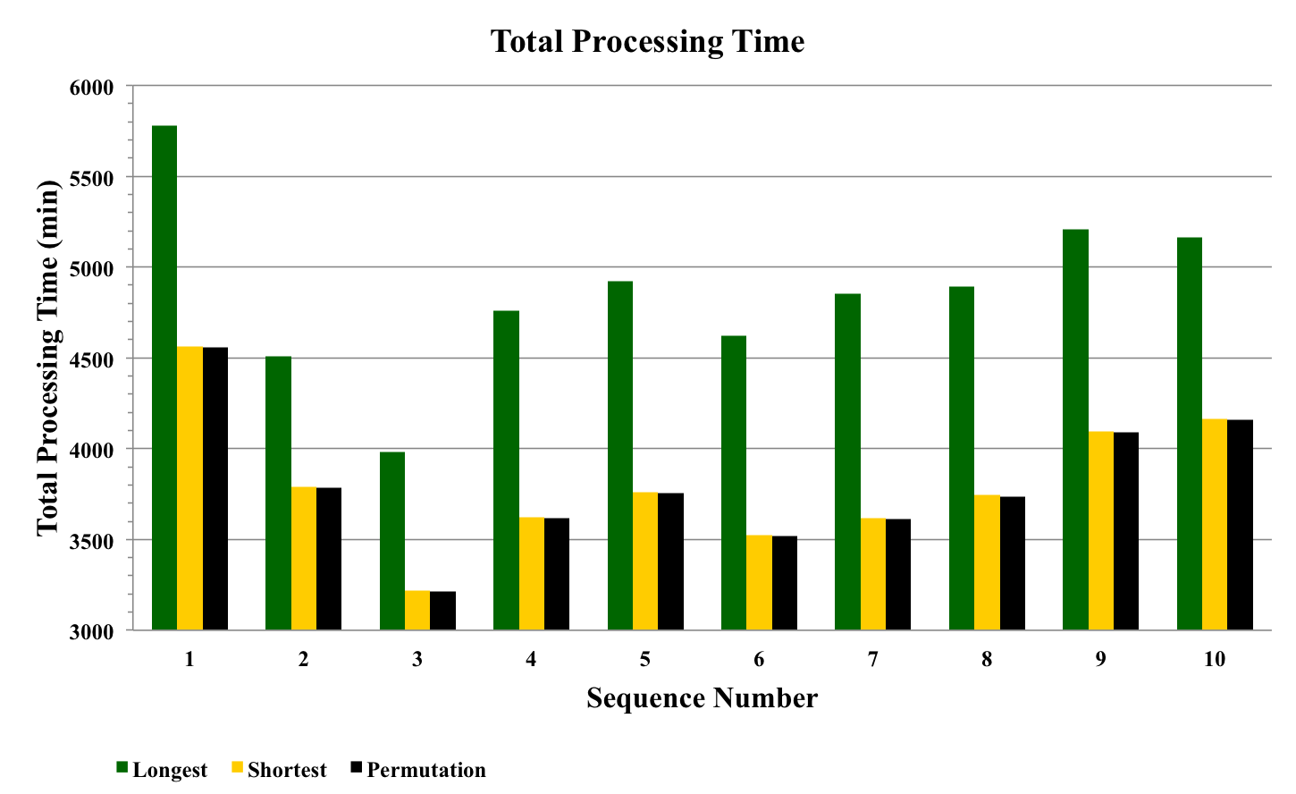
Figure 9.2.2: Total Processing Time

Figure 9.2.3 shows the average remaining life for the last ion source for the same ten sequences compared above. Here, in some cases it seems that the longest greedy algorithm has the highest ion source remaining life. However, the higher remaining life is due to the additional ion source changes, that is, when the ion source was changed close to the completion of the simulation run. For a closer comparison of the data, we calculated the average of all the runs.

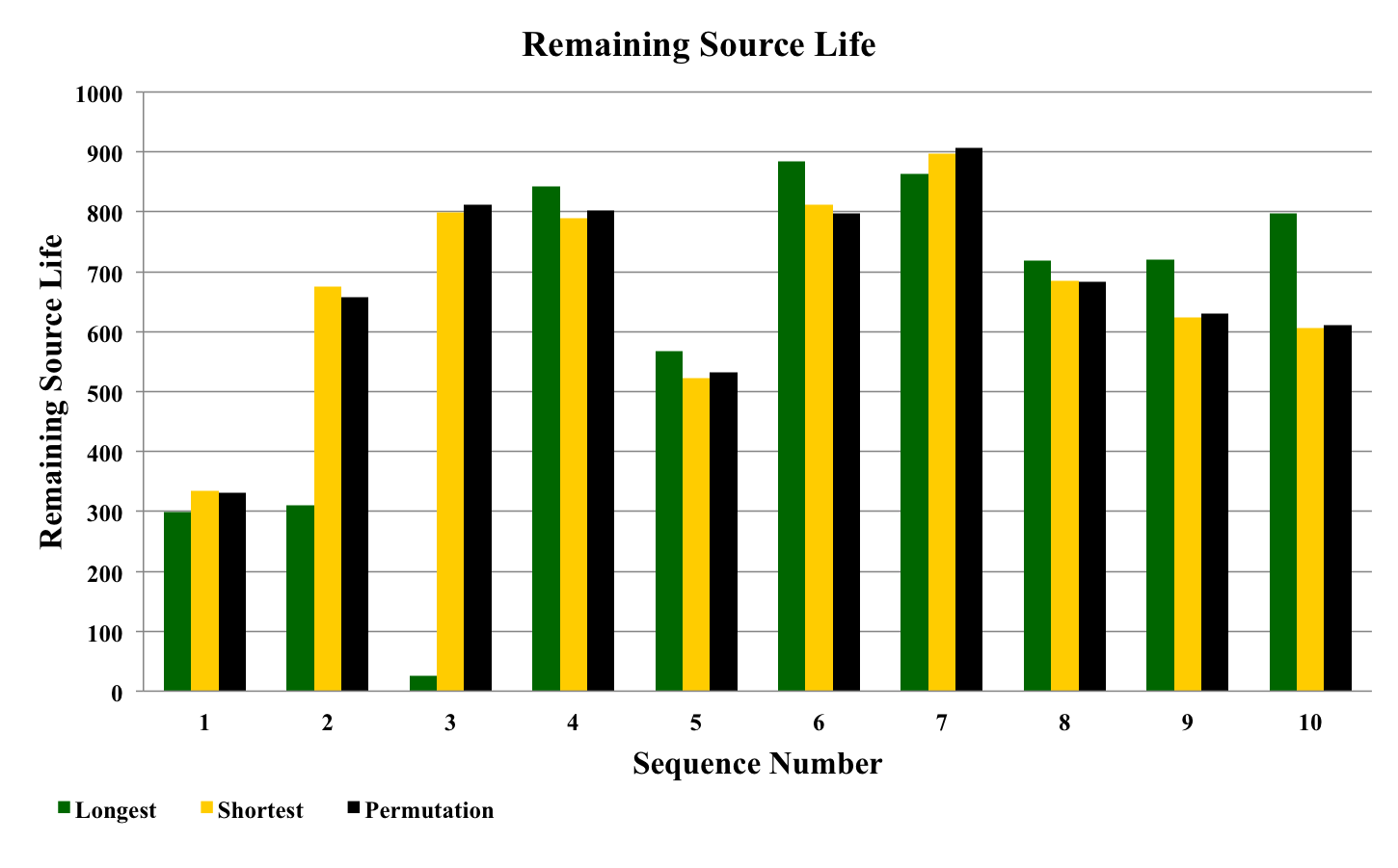
Figure 9.2.3: Remaining Source Life

Table 9.2.7: Average Results for all runs

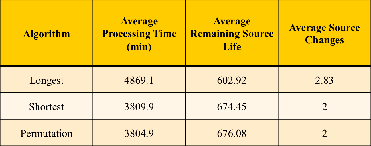
Table 9.2.7 contains the average total processing time as well as the average remaining source life for the ten sequences compared earlier Here it is clear that the longest greedy sequences have the poorest performance. They have the longest total processing times, as well as the lowest remaining source life due to the additional ion source changes. Furthermore, we can see that the results for the shortest greedy and the permutation sequences were very close to each other. This is because both schedules try to minimize the set-up times in between recipes. As a result, the permutation sequences, which have the smallest total set-up times, have the best results both for fastest total processing time, as well as for the highest average ion source remaining life.

We would like to emphasize that this is only a proof of concept analysis; therefore, we are not making any recommendations as to which scheduling algorithm to use. Instead, we are providing a tool that will return data to help planning or scheduling engineers improve their scheduling systems.

Summary

In summary, our simulation tool can be used to:

● Study the benefits of different scheduling techniques

● Test schedules before implementation

● Identify if the current schedule needs adjustments to minimize source changes

● Adjust schedules based on simulation results

● Increase tool availability (Up time)

● Meet manufacturing demands

● And ultimately save money and increase profit

Regardless of the user priorities, our simulation model can be used to study and investigate new or different scheduling logics before implementing them in a real tool.

Tool Recommendations

The simulation model that CTSG has developed is a powerful analysis tool that can be used for many purposes. For example, our model can be used to test different scheduling techniques or methodologies before implementation. This will allow scheduling or planning engineers to show the benefits of a proposed technique to management without the potential dangers of experimental testing.

Additionally, this tool can be used to study any scheduling process that is affected by constraints. One good example are process chambers that need to be maintained after a certain period of time. The tool would provide insight into how to schedule the work to a process chamber and when to perform the necessary maintenance.

Furthermore, this tool can be modified to study more than one tool or machine concurrently. For example, the tool can be expanded to study the scheduling of a group of implant tools (known as a workstation). In the case of implant tools, this type of study would prove beneficial by showing the time savings from a particular scheduling logic that could translate into cost savings. It can also be modified to study other kinds of cluster tools and multiple failures in workstations.

Finally, as a matter of possible future expansions, it may be possible to include deterioration and time into a combined metric to develop more advanced scheduling algorithms. For example, the Permutation algorithm may be modified by splitting repetitions based on deterioration metrics, in order to further extend the ion source’s life. Although, this will increase processing time by increasing set-up times, as was indicated by our sample analysis. The development and analysis of this modified Permutation algorithm with the tool we have developed could be a possible capstone project for future classes.